# 1. 前言
上次讲到基因家族的收缩扩张分析,这次我们以某个节点为切入点,进行特异节点的功能富集分析
其实这篇教程适用于所有的非模式物种 (没有现成的 GO/KEGG 库的物种) 的富集分析
物种特异的比较简单就不进行实践了
# 2. 节点选择
这次选择一个进化上比较重要的节点,水生到陆生的过程,对应进化树为 node25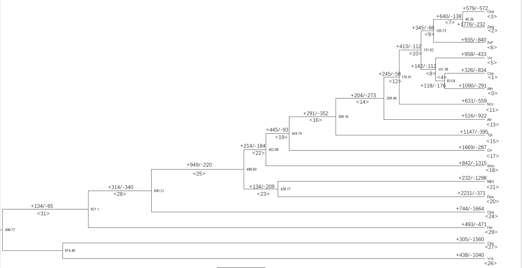
# 3. 获取目的基因
主要是目标基因与背景基因的选择,目标基因可以是该节点显著扩张的基因家族包含的所有物种基因,背景基因一般为该节点包含的 Orthogroup
# 3.1 获取 node25 显著扩张的基因
cat Gamma_p0.05change.tab | cut -f1,27 | grep "+[1-9]" | cut -f1 > node25significant.expand | |
#node25 显著扩张的 orthogroupsID | |
grep -f node0significant.expand Orthogroups.txt |sed "s//\n/g" | grep -E "Ath|Csa|Vvi|Aof|Osa|Zma|Nco|Atr|Tpl|Cri|Smo|Mpo|Ppa" | sort | uniq > node25significant.expand.genes |
目前我们得到了需要进行富集分析的目标基因,接下来是背景基因的选择
# 3.2 node25 背景基因选择
awk 'NR!=1 && $27>0 {print $0}' Gamma_count.tab | cut -f1 > node25.orthogroups | |
#node25 中存在基因的 orthogroupsID | |
grep -f node25.orthogroups Orthogroups.txt |sed "s//\n/g" | grep -E "Ath|Csa|Vvi|Aof|Osa|Zma|Nco|Atr|Tpl|Cri|Smo|Mpo|Ppa" | sort | uniq > node25.genes |
node25.genes 和 node25significant.expand.genes 就是我们进行富集分析所需要的基因号,接下来就是构建背景基因的 GO 和 KEGG 注释,由于是无参物种,所以我们需要自己构建
# 4 背景基因的 GO 和 KEGG 注释
# 4.1 GO/KEGG 注释
使用 eggnog 对背景基因进行注释
seqkit grep -f node25.genes ../../../allpep.fa > node25background.fa | |
# 提取背景基因,需要严格注意基因数是否一致 | |
emapper.py -m diamond -i node25background.fa -o node25 --cpu 16 |
最后我们拿到 node25.emapper.annotations 文件,将前三行和 #删除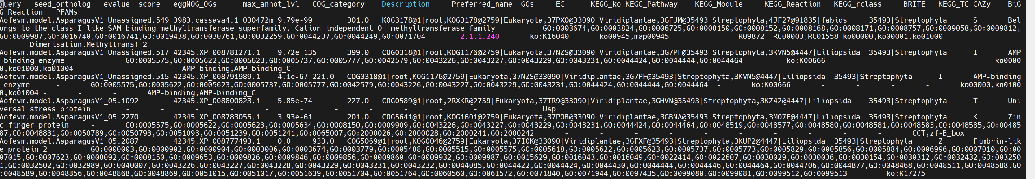
# 4.2 GO 注释库构建
获取 GO 的注释信息:下载地址:http://purl.obolibrary.org/obo/go/go-basic.obo 之后进行修饰
grep "^id:" go-basic.obo |awk '{print $2}' > GO.id | |
grep "^name:" go-basic.obo |awk '{print $2}' > GO.name | |
grep "^namespace:" go-basic.obo |awk '{print $2}' > GO.class | |
paste GO.id GO.name GO.class -d "\t" > GO.library |
文件一共有三列
GO:1903040 exon-exon junction complex assembly biological process | |
GO:1903045 neural crest cell migration involved in sympathetic nervous system development biological process | |
GO:1903046 meiotic cell cycle process biological process | |
GO:1903043 positive regulation of chondrocyte hypertrophy biological process | |
GO:1903044 protein localization to membrane raft biological process | |
GO:1903049 negative regulation of acetylcholine-gated cation channel activity biological process | |
GO:1903047 mitotic cell cycle process biological process | |
GO:1903048 regulation of acetylcholine-gated cation channel activity biological process | |
GO:1903012 positive regulation of bone development biological process | |
GO:1903013 response to differentiation-inducing factor 1 biological process | |
GO:1903010 regulation of bone development biological process | |
GO:1903011 negative regulation of bone development biological process | |
GO:1903016 negative regulation of exo-alpha-sialidase activity biological process | |
GO:1903017 positive regulation of exo-alpha-sialidase activity biological process | |
GO:1903014 cellular response to differentiation-inducing factor 1 biological process | |
GO:1903015 regulation of exo-alpha-sialidase activity biological process | |
GO:1903018 regulation of glycoprotein metabolic process biological process | |
GO:1903019 negative regulation of glycoprotein metabolic process biological process | |
GO:1903020 positive regulation of glycoprotein metabolic process biological process | |
GO:1903023 regulation of ascospore-type prospore membrane assembly biological process |
# 4.3 KEGG 注释库构建
需要下载 ko00001.json: https://www.genome.jp/kegg-bin/get_htext?ko00001
# 需要下载 json 文件 (这是是经常更新的) | |
# https://www.genome.jp/kegg-bin/get_htext?ko00001 | |
# 代码来自:http://www.genek.tv/course/225/task/4861/show | |
library (jsonlite) | |
library (purrr) | |
library (RCurl) | |
library (dplyr) | |
library (stringr) | |
kegg <- function (json = "ko00001.json") { | |
pathway2name <- tibble (Pathway = character (), Name = character ()) | |
ko2pathway <- tibble (Ko = character (), Pathway = character ()) | |
kegg <- fromJSON (json) | |
for (a in seq_along (kegg [["children"]][["children"]])) { | |
A <- kegg [["children"]][["name"]][[a]] | |
for (b in seq_along (kegg [["children"]][["children"]][[a]][["children"]])) { | |
B <- kegg [["children"]][["children"]][[a]][["name"]][[b]] | |
for (c in seq_along (kegg [["children"]][["children"]][[a]][["children"]][[b]][["children"]])) { | |
pathway_info <- kegg [["children"]][["children"]][[a]][["children"]][[b]][["name"]][[c]] | |
pathway_id <- str_match (pathway_info, "ko [0-9]{5}")[1] | |
pathway_name <- str_replace (pathway_info, "\\[PATH:ko [0-9]{5}\\]", "") %>% str_replace ("[0-9]{5} ","") | |
pathway2name <- rbind (pathway2name, tibble (Pathway = pathway_id, Name = pathway_name)) | |
kos_info <- kegg [["children"]][["children"]][[a]][["children"]][[b]][["children"]][[c]][["name"]] | |
kos <- str_match (kos_info, "K [0-9]*")[,1] | |
ko2pathway <- rbind (ko2pathway, tibble (Ko = kos, Pathway = rep (pathway_id, length (kos)))) | |
} | |
} | |
} | |
colnames (ko2pathway) <- c ("KO","Pathway") | |
save (pathway2name, ko2pathway, file = "kegg_info.RData") | |
write.table (pathway2name,"KEGG.library",sep="\t",row.names = F) | |
} | |
kegg (json = "ko00001.json") |
# 4.4 背景注释构建
主要是将自己的基因集与注释库结合
library (clusterProfiler) | |
library (dplyr) | |
library (stringr) | |
options (stringsAsFactors = F) | |
##===============================STEP1:GO 注释生成 ======================= | |
# 自己构建的话,首先需要读入文件 | |
egg <- read.delim ("node25.emapper.annotations",header = T,sep="\t") | |
egg [egg==""]<-NA #将空行变成 NA,方便下面的去除 | |
# 从文件中挑出基因 query 与 eggnog 注释信息 | |
##gene_info <- egg %>% | |
## dplyr::select (GID = query, GENENAME = eggNOG_OGs) %>% na.omit () | |
# 挑出 query_name 与 GO 注释信息 | |
gterms <- egg %>% | |
dplyr::select (query, GOs) %>% na.omit () | |
gene_ids <- egg$query | |
eggnog_lines_with_go <- egg$GOs!= "" | |
eggnog_lines_with_go | |
eggnog_annoations_go <- str_split (egg [eggnog_lines_with_go,]$GOs, ",") | |
gene2go <- data.frame (gene = rep (gene_ids [eggnog_lines_with_go], | |
times = sapply (eggnog_annoations_go, length)), | |
term = unlist (eggnog_annoations_go)) | |
names (gene2go) <- c ('gene_id', 'ID') | |
go2name <- read.delim ('GO.library', header = FALSE, stringsAsFactors = FALSE) | |
names (go2name) <- c ('ID', 'Description', 'Ontology') | |
go_anno <- merge (gene2go, go2name, by = 'ID', all.x = TRUE) | |
## 将 GO 注释信息保存 | |
save (go_anno,file = "node25_GO.rda") | |
##===============================STEP2:KEGG 注释生成 ======================= | |
gene2ko <- egg %>% | |
dplyr::select (GID = query, KO = KEGG_ko) %>% | |
na.omit () | |
pathway2name <- read.delim ("KEGG.library") | |
colnames (pathway2name)<-c ("Pathway","Name") | |
gene2ko$KO <- str_replace (gene2ko$KO, "ko:","") | |
gene2pathway <- gene2ko %>% left_join (ko2pathway, by = "KO") %>% | |
dplyr::select (GID, Pathway) %>% | |
na.omit () | |
kegg_anno<- merge (gene2pathway,pathway2name,by = 'Pathway', all.x = TRUE)[,c (2,1,3)] | |
colnames (kegg_anno) <- c ('gene_id','pathway_id','pathway_description') | |
save (kegg_anno,file = "node25_KEGG.rda") |
# 4.5 GO/KEEG 富集分析
利用生成的 node25_GO.rda、node25_KEGG.rda、以及之前的 node25significant.expand.genes 文件进行富集分析
我在分析的时候没有设置 p 的阈值,输出了所有的富集结果,毕竟作图也只需要 TOP10 或者 TOP20,大家按照需求设定
##===============================STEP3:GO 富集分析 ================= | |
# 目标基因列表 (全部基因) | |
gene_select <- read.delim (file = 'node25significant.expand.genes', stringsAsFactors = FALSE,header = F)$V1 | |
#GO 富集分析 | |
# 默认以所有注释到 GO 的基因为背景集,也可通过 universe 参数输入背景集 | |
# 默认以 p<0.05 为标准,Benjamini 方法校正 p 值,q 值阈值 0.2 | |
# 默认输出 top500 富集结果 | |
# 如果想输出所有富集结果(不考虑 p 值阈值等),将 p、q 等值设置为 1 即可 | |
# 或者直接在 enrichResult 类对象中直接提取需要的结果 | |
go_rich <- enricher (gene = gene_select, | |
TERM2GENE = go_anno [c ('ID', 'gene_id')], | |
TERM2NAME = go_anno [c ('ID', 'Description')], | |
pvalueCutoff = 1, | |
pAdjustMethod = 'BH', | |
qvalueCutoff = 1 | |
) | |
# 输出默认结果,即根据上述 p 值等阈值筛选后的 | |
tmp <- merge (go_rich, go2name [c ('ID', 'Ontology')], by = 'ID') | |
tmp <- tmp [c (10, 1:9)] | |
tmp <- tmp [order (tmp$pvalue), ] | |
write.table (tmp, 'node6expand.xls', sep = '\t', row.names = FALSE, quote = FALSE) | |
##===============================STEP4:KEGG 注释 ================= | |
gene_select <- read.delim ('node25significant.expand.genes', stringsAsFactors = FALSE,header = F)$V1 | |
#KEGG 富集分析 | |
# 默认以所有注释到 KEGG 的基因为背景集,也可通过 universe 参数指定其中的一个子集作为背景集 | |
# 默认以 p<0.05 为标准,Benjamini 方法校正 p 值,q 值阈值 0.2 | |
# 默认输出 top500 富集结果 | |
kegg_rich <- enricher (gene = gene_select, | |
TERM2GENE = kegg_anno [c ('pathway_id', 'gene_id')], | |
TERM2NAME = kegg_anno [c ('pathway_id', 'pathway_description')], | |
pvalueCutoff = 1, | |
pAdjustMethod = 'BH', | |
qvalueCutoff = 1, | |
maxGSSize = 500) | |
# 输出默认结果,即根据上述 p 值等阈值筛选后的 | |
write.table (kegg_rich, 'node25significant.expand.KEGG.xls', sep = '\t', row.names = FALSE, quote = FALSE) |
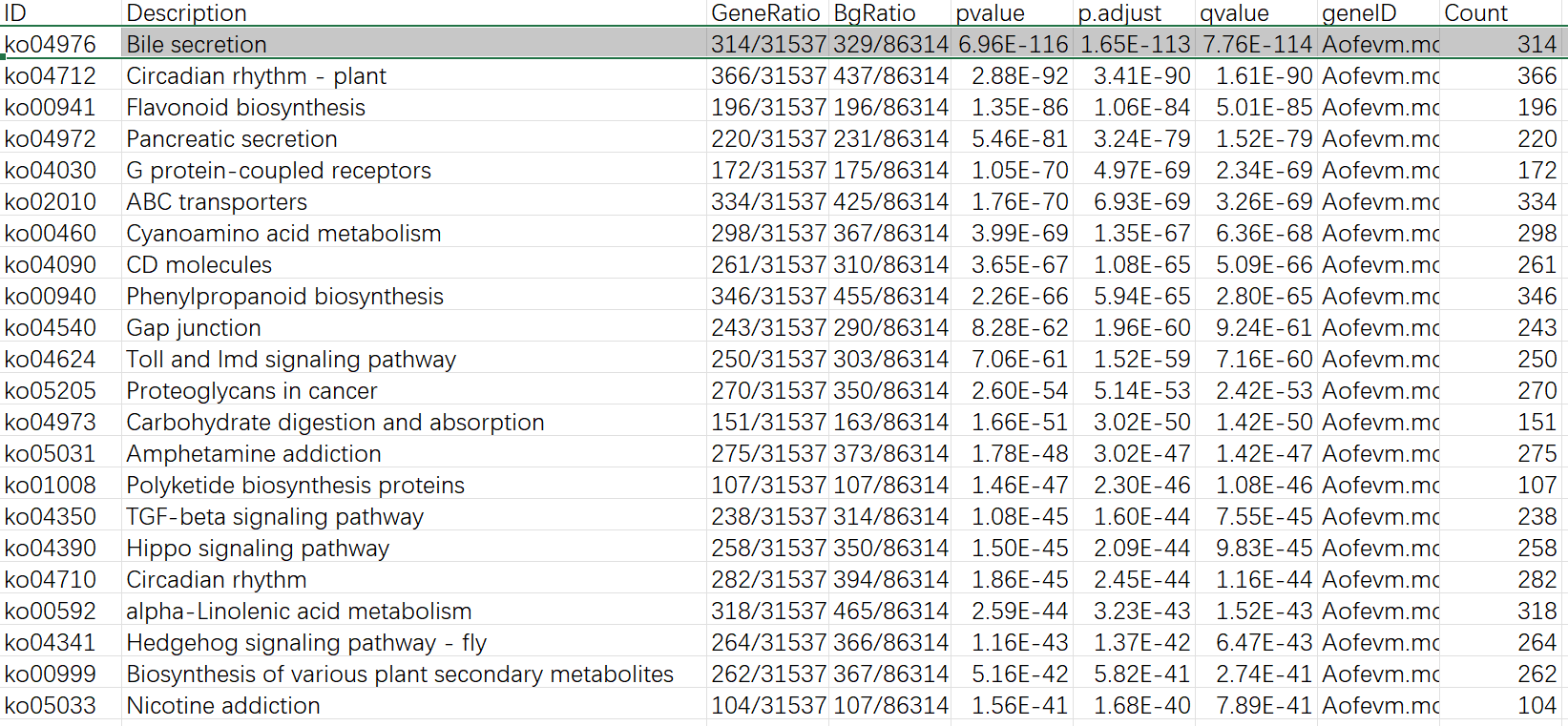
需要注意生成的文件中有一些 term 可能是重复的,比如 GO 富集结果的 16,17 行,仔细看 geneID 那一列就会发现两行的基因是完全一样的,需要删掉一个。还有一点就是在 GO/KEGG 富集的结果中,有一些是动物相关的 (KEGG 结果的第一行),这些也请酌情考虑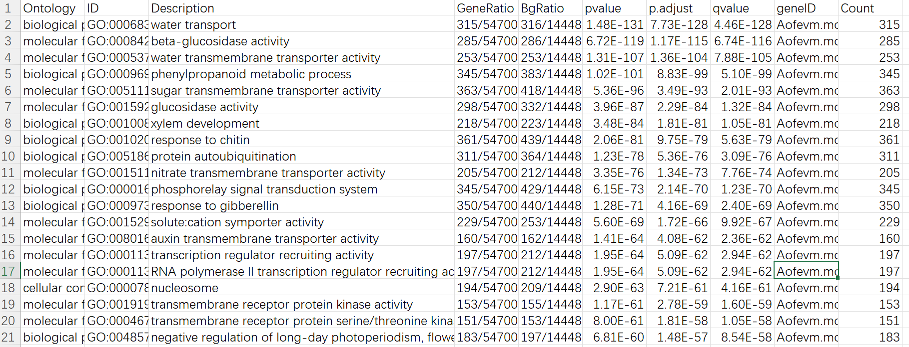
# 5 GO/KEGG 绘图
此次使用 TOP10 的 term 进行绘图,看一下在陆生植物出现的关键进化节点主要是哪些基因功能发生了大规模扩张
library (ggplot2) | |
pathway = read.delim ("node25significant.expand.GO.xls",header = T,sep="\t") | |
pathway$GeneRatio<- pathway [,10]/54700 ## 这个 54700 是 GeneRatio 的那个数值,自己修改 | |
pathway$log<- -log10 (pathway [,6]) | |
library (dplyr) | |
library (ggrepel) | |
GO <- arrange (pathway,pathway [,6]) | |
GO_dataset <- GO [1:10,] | |
# 按照 PValue 从低到高排序 [升序] | |
GO_dataset$Description<- factor (GO_dataset$Description,levels = rev (GO_dataset$Description)) | |
GO_dataset$GeneRatio <- as.numeric (GO_dataset$GeneRatio) | |
GO_dataset$GeneRatio | |
GO_dataset$log | |
# 图片背景设定 | |
mytheme <- theme (axis.title=element_text (face="bold", size=8,colour = 'black'), #坐标轴标题 | |
axis.text.y = element_text (face="bold", size=6,colour = 'black'), #坐标轴标签 | |
axis.text.x = element_text (face ="bold",color="black",angle=0,vjust=1,size=8), | |
axis.line = element_line (size=0.5, colour = 'black'), #轴线 | |
panel.background = element_rect (color='black'), #绘图区边框 | |
plot.title = element_text (face="bold", size=8,colour = 'black',hjust = 0.8), | |
legend.key = element_blank () #关闭图例边框 | |
) | |
# 绘制 GO 气泡图 | |
p <- ggplot (GO_dataset,aes (x=GeneRatio,y=Description,colour=log,size=Count,shape=Ontology))+ | |
geom_point ()+ | |
scale_size (range=c (2, 8))+ | |
scale_colour_gradient (low = "#52c2eb",high = "#EA4F30")+ | |
theme_bw ()+ | |
labs (x='Fold Enrichment',y='GO Terms', #自定义 x、y 轴、标题内容 | |
title = 'Enriched GO Terms')+ | |
labs (color=expression (-log [10](pvalue)))+ | |
theme (legend.title=element_text (size=8), legend.text = element_text (size=14))+ | |
theme (axis.title.y = element_text (margin = margin (r = 50)),axis.title.x = element_text (margin = margin (t = 20)))+ | |
theme (axis.text.x = element_text (face ="bold",color="black",angle=0,vjust=1)) | |
plot <- p+mytheme | |
plot | |
# 保存图片 | |
ggsave (plot,filename = "node25GO.pdf",width = 210,height = 210,units = "mm",dpi=300) | |
ggsave (plot,filename = "node25GO.png",width = 210,height = 210,units = "mm",dpi=300) |
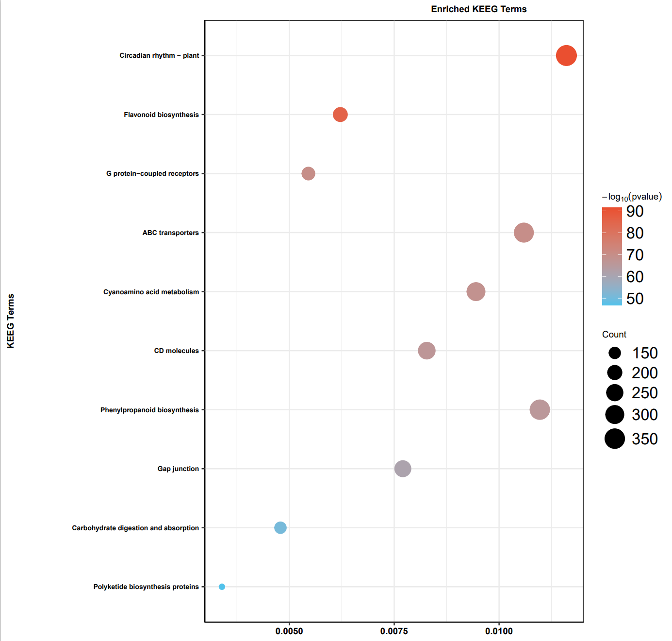
KEGG 同理,大家修改运行参数和输入文件即可
pathway = read.delim ("node25significant.expand.KEGG.xls",header = T,sep="\t") | |
pathway$GeneRatio<- pathway [,9]/31537 | |
pathway$log<- -log10 (pathway [,5]) | |
library (dplyr) | |
library (ggrepel) | |
GO <- arrange (pathway,pathway [,5]) | |
GO_dataset <- GO [1:10,] | |
#Pathway 列最好转化成因子型,否则作图时 ggplot2 会将所有 Pathway 按字母顺序重排序 | |
# 将 Pathway 列转化为因子型 | |
GO_dataset$Description<- factor (GO_dataset$Description,levels = rev (GO_dataset$Description)) | |
GO_dataset$GeneRatio <- as.numeric (GO_dataset$GeneRatio) | |
GO_dataset<- arrange (GO_dataset,GO_dataset [,5]) | |
GO_dataset$GeneRatio | |
GO_dataset$log | |
# 图片背景设定 | |
mytheme <- theme (axis.title=element_text (face="bold", size=8,colour = 'black'), #坐标轴标题 | |
axis.text.y = element_text (face="bold", size=6,colour = 'black'), #坐标轴标签 | |
axis.text.x = element_text (face ="bold",color="black",angle=0,vjust=1,size=8), | |
axis.line = element_line (size=0.5, colour = 'black'), #轴线 | |
panel.background = element_rect (color='black'), #绘图区边框 | |
plot.title = element_text (face="bold", size=8,colour = 'black',hjust = 0.8), | |
legend.key = element_blank () #关闭图例边框 | |
) | |
# 绘制 KEGG 气泡图 | |
p <- ggplot (GO_dataset,aes (x=GeneRatio,y=Description,colour=log,size=Count))+ | |
geom_point ()+ | |
scale_size (range=c (2, 8))+ | |
scale_colour_gradient (low = "#52c2eb",high = "#EA4F30")+ | |
theme_bw ()+ | |
labs (x='Fold Enrichment',y='KEEG Terms', #自定义 x、y 轴、标题内容 | |
title = 'Enriched KEEG Terms')+ | |
labs (color=expression (-log [10](pvalue)))+ | |
theme (legend.title=element_text (size=8), legend.text = element_text (size=14))+ | |
theme (axis.title.y = element_text (margin = margin (r = 50)),axis.title.x = element_text (margin = margin (t = 20)))+ | |
theme (axis.text.x = element_text (face ="bold",color="black",angle=0,vjust=1)) | |
plot <- p+mytheme | |
plot | |
# 保存图片 | |
ggsave (plot,filename = "node25KEGG.pdf",width = 210,height = 210,units = "mm",dpi=300) | |
ggsave (plot,filename = "node25KEGG.png",width = 210,height = 210,units = "mm",dpi=300) |
最后我们可以看到,在 GO 富集中,最显著的是水运输相关功能,KEGG 富集中,最显著的是昼夜节律,大家觉得陆生植物的进化和这两个功能有没有关系?欢迎讨论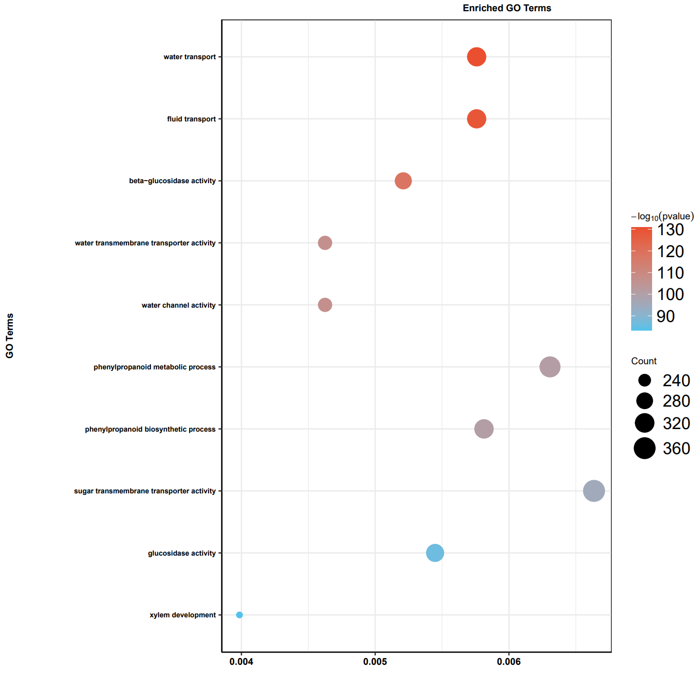
# 6 结果整理
结合这三篇推文的结果,我们可以整理一张主图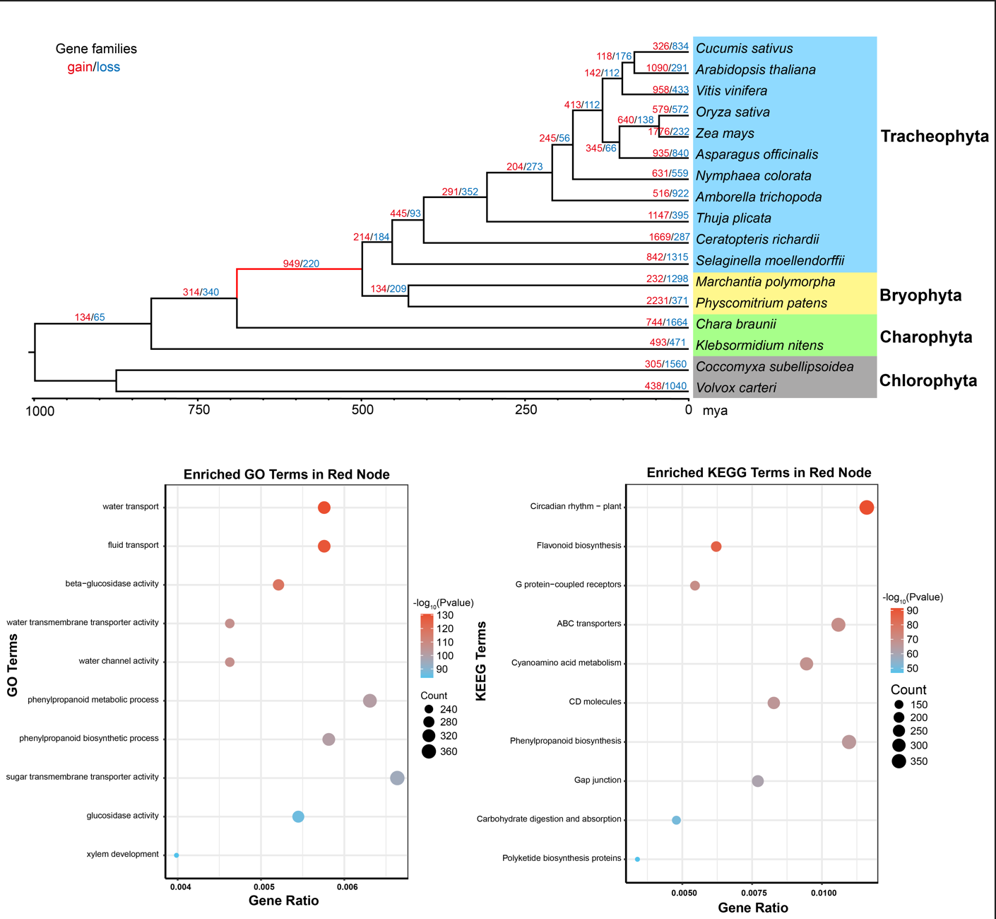
# 总结
== 比较基因组学分析的基本内容已经介绍完了,如果说有遗漏的内容那应该就是加倍化事件,由于本次使用的数据集跨度过大所以没有增加 WGD 的分析,大家有什么问题欢迎交流 ==