# 前言
最近有幸加入生信技能树的单细胞数据挖掘尝鲜群,借此机会给大家分享一下
生信技能树单细胞数据挖掘笔记 (2):创建 Seurat 对象并进行质控、筛选高变基因并可视化
生信技能树单细胞数据挖掘笔记 (4):其他分析(周期判断、double 诊断、细胞类型注释)
# 课程大纲
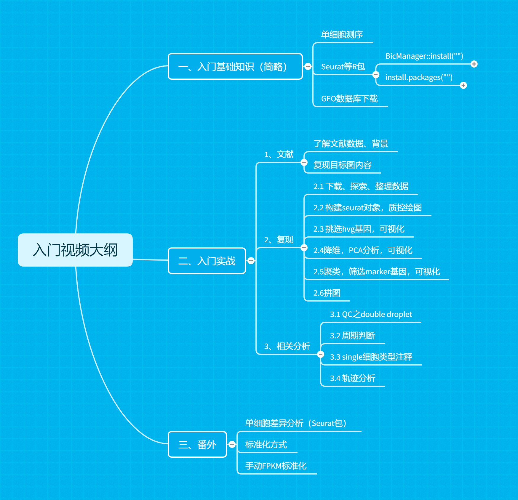
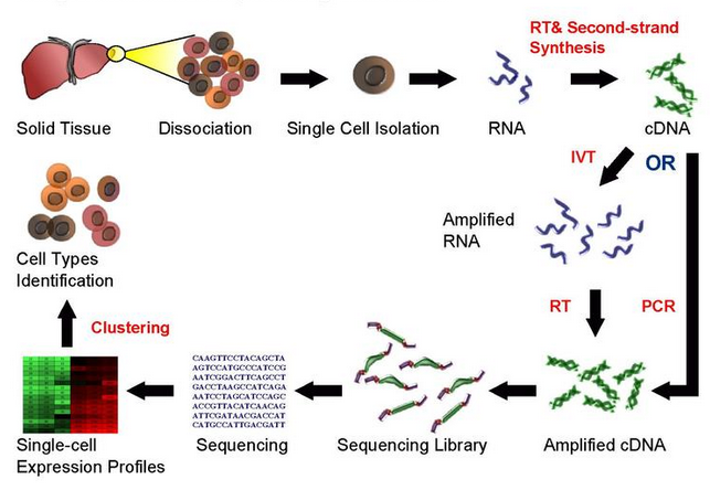
# 入门基础知识
所需 R 包
getOption ("BioC_mirror") | |
getOption ("CRAN") | |
#CRAN 基础包 | |
options (CRAN="https://mirrors.ustc.edu.cn/CRAN/")## 设置镜像 | |
cran_packages <- c ('tidyverse', | |
'ggplot2' | |
) | |
for (pkg in cran_packages){ | |
if (! require (pkg,character.only=T) ) { | |
install.packages (pkg,ask = F,update = F) | |
require (pkg,character.only=T) | |
} | |
} | |
if (!require ("BiocManager")) install.packages ("BiocManager",update = F,ask = F) | |
#Bio 分析包 | |
Biocductor_packages <- c ("Seurat", | |
"scran", | |
"scater", | |
"monocle", | |
"DropletUtils", | |
"SingleR" | |
) | |
options (BioC_mirror="https://mirrors.ustc.edu.cn/bioc/") | |
#options (BioC_mirror="https://mirrors.tuna.tsinghua.edu.cn/bioconductor") | |
# use BiocManager to install | |
for (pkg in Biocductor_packages){ | |
if (! require (pkg,character.only=T) ) { | |
BiocManager::install (pkg,ask = F,update = F) | |
require (pkg,character.only=T) | |
} | |
} | |
# 最后检查下成功与否 | |
for (pkg in c (Biocductor_packages,cran_packages)){ | |
require (pkg,character.only=T) | |
} | |
### GEO | |
# | |
# GEO Platform (GPL) | |
# GEO Sample (GSM) | |
# GEO Series (GSE) | |
# GEO Dataset (GDS) | |
# 一篇文章可以有一个或者多个 GSE 数据集,一个 GSE 里面可以有一个或者多个 GSM 样本。 | |
# 多个研究的 GSM 样本可以根据研究目的整合为一个 GDS,不过 GDS 本身用的很少。 | |
# 而每个数据集都有着自己对应的芯片平台,就是 GPL。(芯片名与基因名 ID 转换) | |
#https://blog.csdn.net/weixin_43569478/article/details/108079337 | |
# https://www.ncbi.nlm.nih.gov/geo/query/acc.cgi?acc= | |
BiocManager::install ("GEOquery") | |
library (GEOquery) | |
gse1009 <- getGEO ('GSE1009', destdir=".") | |
class (gse1009) | |
length (gse1009) | |
a <- gse1009 [[1]] | |
class (gse1009 [1]) | |
a | |
b <- exprs (a) | |
c <- pData (a) | |
a$platform_id |
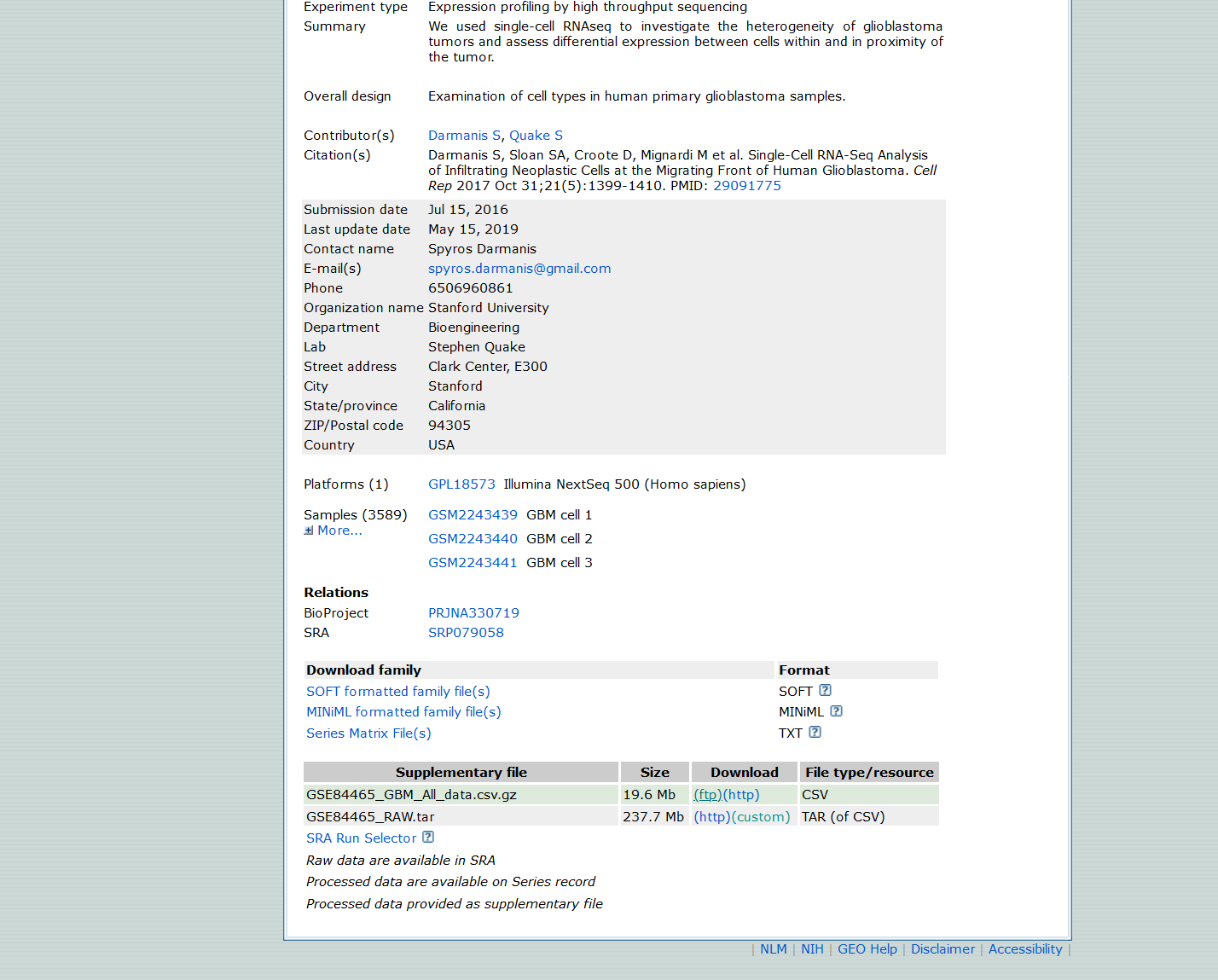
# 下载、探索、数据整理
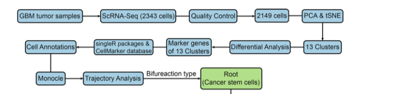
本次数据采用《Glioblastoma cell differentiation trajectory predicts the immunotherapy response and overall survival of patients》中的单细胞数据进行分析(GSE 号:84465)

### 1、下载、探索、整理数据 ---- | |
## 1.1 下载、探索数据 | |
#https://www.ncbi.nlm.nih.gov/geo/query/acc.cgi?acc=GSE84465 ## 数据来源 | |
sessionInfo () |
# 读取数据
a <- read.table ("../rawdata/GSE84465_GBM_All_data.csv.gz") | |
a [1:4,1:4] | |
# 行名为 symbol ID | |
# 列名为 sample,看上去像是两个元素的组合。 | |
summary (a [,1:4]) | |
boxplot (a [,1:4]) | |
head (rownames (a)) | |
tail (rownames (a),10) | |
# 可以看到原文的 counts 矩阵来源于 htseq 这个计数软件,所以有一些不是基因的行需要剔除: | |
# "no_feature" "ambiguous" "too_low_aQual" "not_aligned" "alignment_not_unique" | |
tail (a [,1:4],10) | |
a=a [1:(nrow (a)-5),] | |
# 原始 counts 数据 | |
#3,589 cells of 4 human primary GBM samples, accession number GSE84465 | |
#2,343 cells from tumor cores and 1,246 cells from peripheral regions | |
b <- read.table ("../rawdata/SraRunTable.txt", | |
sep = ",", header = T) | |
b [1:4,1:4] | |
table (b$Patient_ID) # 4 human primary GBM samples | |
table (b$TISSUE) # tumor cores and peripheral regions | |
table (b$TISSUE,b$Patient_ID) |
# 整理数据
可以发现两个数据不对应,a 矩阵行名(sample)并非为 GSM 编号,而主要是由相应的 plate_id 与 Well 组合而成
## 1.2 整理数据 | |
# tumor and peripheral 分组信息 | |
head (colnames (a)) | |
[1] "X1001000173.G8" "X1001000173.D4" "X1001000173.B4" "X1001000173.A2" "X1001000173.E2" "X1001000173.F6" | |
head (b$plate_id) | |
[1] 1001000173 1001000173 1001000173 1001000173 1001000173 1001000173 | |
head (b$Well) | |
#a 矩阵行名(sample)并非为 GSM 编号,而主要是由相应的 plate_id 与 Well 组合而成 | |
b.group <- b [,c ("plate_id","Well","TISSUE","Patient_ID")] | |
b.group$sample <- paste0 ("X",b.group$plate_id,".",b.group$Well) | |
head (b.group) | |
plate_id Well TISSUE Patient_ID sample | |
1 1001000173 G8 Tumor BT_S2 X1001000173.G8 | |
2 1001000173 D4 Tumor BT_S2 X1001000173.D4 | |
3 1001000173 B4 Tumor BT_S2 X1001000173.B4 | |
4 1001000173 A2 Tumor BT_S2 X1001000173.A2 | |
5 1001000173 E2 Tumor BT_S2 X1001000173.E2 | |
6 1001000173 F6 Tumor BT_S2 X1001000173.F6 | |
identical (colnames (a),b.group$sample) | |
# 筛选 tumor cell | |
index <- which (b.group$TISSUE=="Tumor") | |
length (index) | |
group <- b.group [index,] #筛选的是行 | |
head (group) | |
a.filt <- a [,index] #筛选的是列 | |
dim (a.filt) | |
identical (colnames (a.filt),group$sample) |
经过筛选之后得到所有的肿瘤细胞的表达矩阵