单细胞实战 (4)：STAR 与 cellranger 结果比较 - 单细胞 - 生信学习 | Zhou Xiaozhao = 小钊の笔记 = 前天是小兔子，昨天是小鹿，今天是你

# 前言

本次主要使用 Seurat 比较 STAR 与 Cellranger 的输出结果，只会进行简单的聚类工作。

# 数据读入

	> library (Seurat)
	> library (dplyr)
	> library (magrittr)
	> library (gtools)
	> library (stringr)
	> library (Matrix)
	> setwd ("D://data/ScRNAcode")
	## 读入 STAR 数据
	> matrix.dir="STAR/"
	> barcode.path <- paste0 (matrix.dir,"barcodes.tsv")
	> features.path <- paste0 (matrix.dir,"features.tsv")
	> matrix.path <- paste0 (matrix.dir, "matrix.mtx")
	> STARmatrix <- readMM (file = matrix.path)
	> feature.names = read.delim (features.path,
	+ header = FALSE,
	+ stringsAsFactors = FALSE)
	> barcode.names = read.delim (barcode.path,
	+ header = FALSE,
	+ stringsAsFactors = FALSE)
	> colnames (STARmatrix) = barcode.names$V1
	> rownames (STARmatrix) = feature.names$V2
	> STARmatrix<-as.matrix (STARmatrix)
	> STARmatrix [1:6,1:6]
	## 创建 seurat 对象
	## 创建 STAR 的 Seurat 对象
	> STAR <- CreateSeuratObject (STARmatrix,project = "zsz",
	min.cells = 3, min.features = 200)
	## 创建 Cellranger 的 Seurat 对象
	> dir="cellranger/"
	> counts <- Read10X (data.dir = dir)
	> RANGER <- CreateSeuratObject (counts, project = "zsz",
	min.cells=3, min.features = 200)

# 数据比较

	> ## 数据比较
	> dim (STARmatrix)
	[1] 33538 2048
	> dim (counts)
	[1] 33538 2112
	> dim (STAR)
	[1] 13350 2046
	> dim (RANGER)
	[1] 13314 2105
	> fivenum (apply (STARmatrix,1,function (x) sum (x>0)))
	MIR1302-2HG IGFBPL1 AL008723.2 FXYD7 MT-CO1
	0 0 0 29 2047
	> fivenum (apply (counts,1,function (x) sum (x>0)))
	MIR1302-2HG FAM221B LINC01638 DGKE MT-CO1
	0 0 0 29 2108
	> pdf ("box.pdf",height = 9,width = 9)
	> boxplot (apply (STARmatrix,1,function (x) sum (x>0) ),main = "STAR",col = "lightgray")
	> boxplot (apply (counts,1,function (x) sum (x>0) ),main = "Cellranger",col = "lightgray")
	> dev.off ()
	RStudioGD
	2
	> pdf ("hist.pdf",height = 9,width = 9)
	> hist (apply (STARmatrix,2,function (x) sum (x>0) ),col = "lightgray",
	+ breaks=20,xlim=c (0,4000),ylim=c (0,800),
	+ labels=F,main="STAR",
	+ xlab="genes",ylab="cells")
	> abline (v=median (apply (STARmatrix,2,function (x) sum (x>0))),col='red')
	> hist (apply (counts,2,function (x) sum (x>0) ),col = "lightgray",
	+ breaks=20,xlim=c (0,4000),ylim=c (0,800),
	+ labels=F,main="Cellranger",
	+ xlab="genes",ylab="cells")
	> abline (v=median (apply (counts,2,function (x) sum (x>0))),col='red')
	> dev.off ()

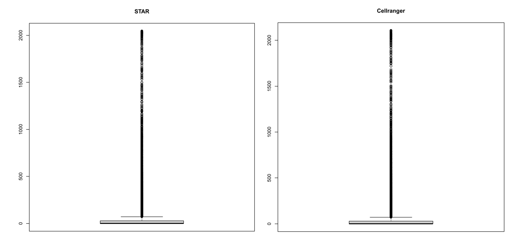
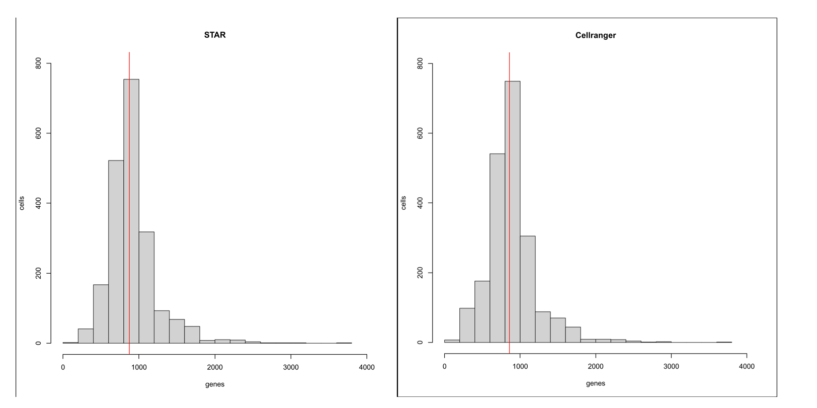
根据箱线图，直方图和矩阵的基本信息，可以看到 STAR 与 cellranger 的结果差距很小

# 质量控制与聚类比较

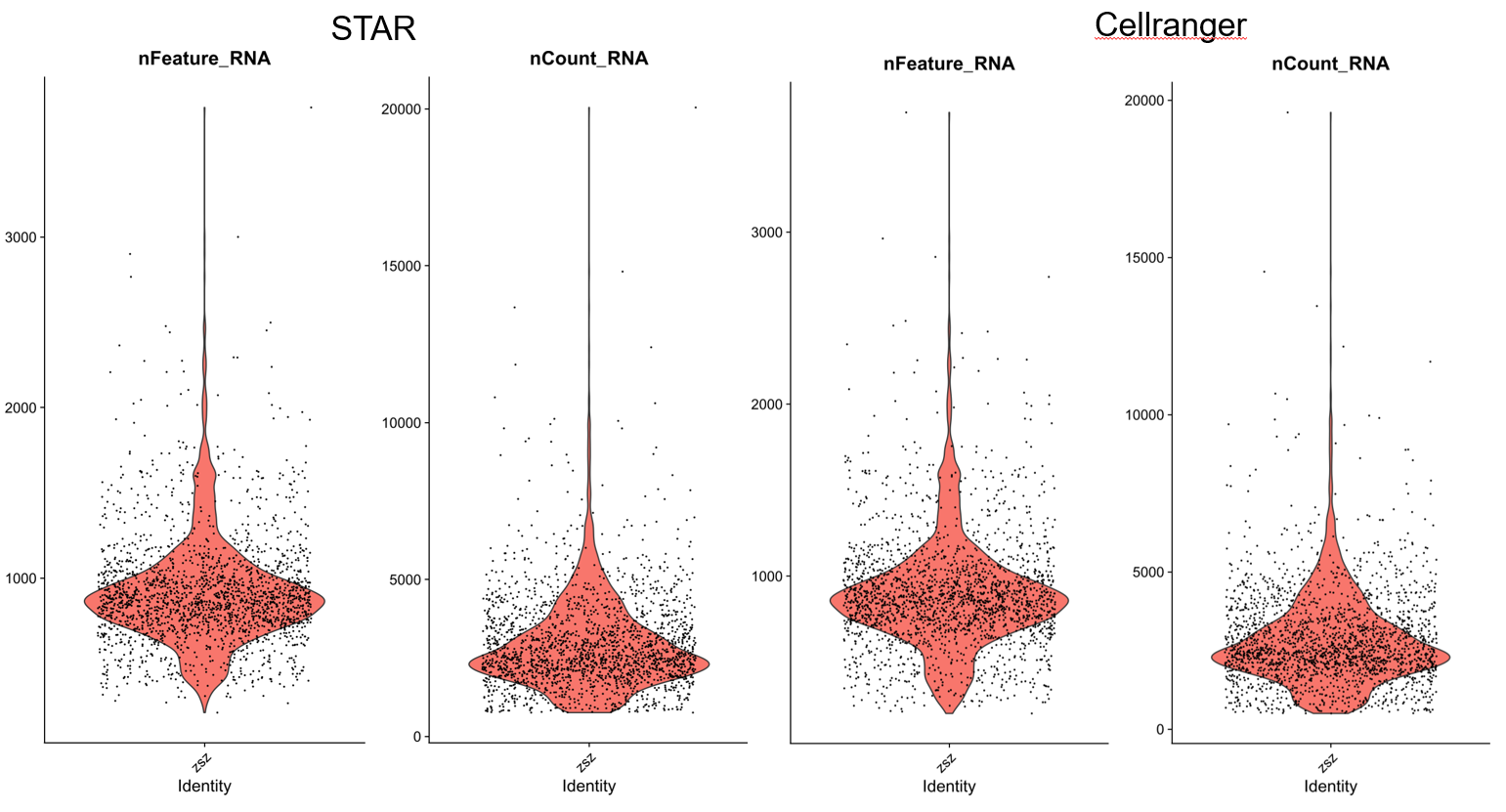
	> pdf("qc.pdf",height = 9,width = 9)
	> VlnPlot(STAR,
	+ features = c("nFeature_RNA", "nCount_RNA"),
	+ pt.size = 0.1,
	+ ncol = 2)
	> VlnPlot(RANGER,
	+ features = c("nFeature_RNA", "nCount_RNA"),
	+ pt.size = 0.1,
	+ ncol = 2)
	> dev.off()
	RStudioGD
	2

	> STAR<-subset(STAR,subset=nFeature_RNA>500 & nFeature_RNA<2000)
	> STAR <- NormalizeData(STAR, normalization.method = "LogNormalize", scale.factor = 10000)
	Performing log-normalization
	0% 10 20 30 40 50 60 70 80 90 100%
	[----\|----\|----\|----\|----\|----\|----\|----\|----\|----\|
	**************************************************\|
	> table(STAR@meta.data$orig.ident)

	zsz
	1896
	> STAR <- FindVariableFeatures(STAR, selection.method = "vst", nfeatures = 2000)
	Calculating gene variances
	0% 10 20 30 40 50 60 70 80 90 100%
	[----\|----\|----\|----\|----\|----\|----\|----\|----\|----\|
	**************************************************\|
	Calculating feature variances of standardized and clipped values
	0% 10 20 30 40 50 60 70 80 90 100%
	[----\|----\|----\|----\|----\|----\|----\|----\|----\|----\|
	**************************************************\|
	> top10 <- head(VariableFeatures(STAR), 10)
	> top10
	[1] "S100A9" "S100A8" "IGLC2" "IGKC" "LYZ" "IGLC3" "CCL3" "NFKBIA" "PTGDS" "S100A12"

	> RANGER<-subset(RANGER,subset=nFeature_RNA>500 & nFeature_RNA<2000)
	> RANGER<- NormalizeData(RANGER, normalization.method = "LogNormalize", scale.factor = 10000)
	Performing log-normalization
	0% 10 20 30 40 50 60 70 80 90 100%
	[----\|----\|----\|----\|----\|----\|----\|----\|----\|----\|
	**************************************************\|
	> table(RANGER@meta.data$orig.ident)

	zsz
	1895
	> RANGER <- FindVariableFeatures(RANGER, selection.method = "vst", nfeatures = 2000)
	Calculating gene variances
	0% 10 20 30 40 50 60 70 80 90 100%
	[----\|----\|----\|----\|----\|----\|----\|----\|----\|----\|
	**************************************************\|
	Calculating feature variances of standardized and clipped values
	0% 10 20 30 40 50 60 70 80 90 100%
	[----\|----\|----\|----\|----\|----\|----\|----\|----\|----\|
	**************************************************\|
	> top10 <- head(VariableFeatures(RANGER), 10)
	> top10
	[1] "S100A9" "S100A8" "IGLC2" "IGKC" "LYZ" "CCL3" "NFKBIA" "IGLC3" "PTGDS" "S100A12"

	> scale.genes <- rownames(STAR)
	> STAR <- ScaleData(STAR, features = scale.genes)
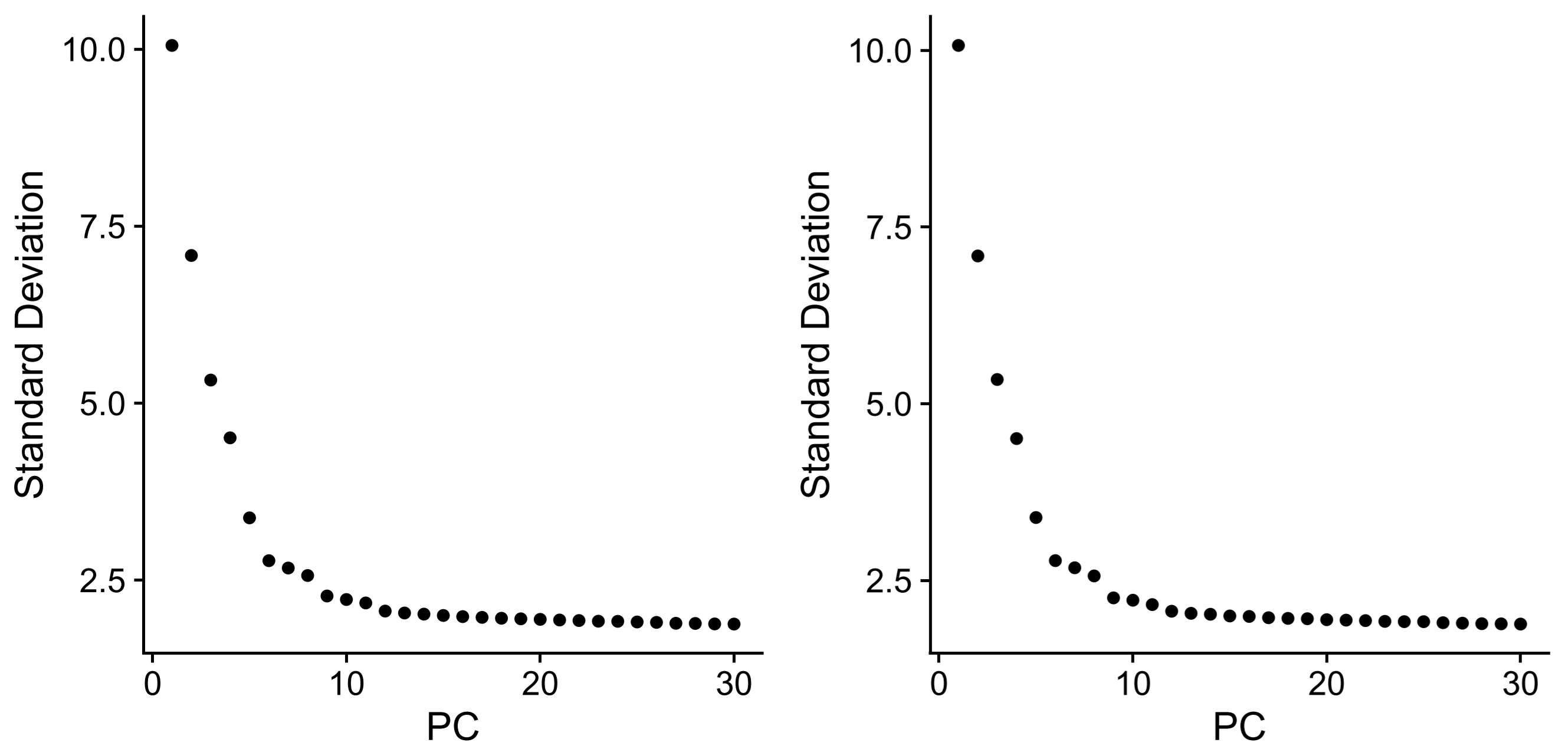
	> STAR <- RunPCA(STAR, features = VariableFeatures(STAR))
	> plot1 <- ElbowPlot(STAR, ndims=30, reduction="pca")
	> scale.genes <- rownames(RANGER)
	> RANGER <- ScaleData(RANGER, features = scale.genes)
	> RANGER <- RunPCA(RANGER, features = VariableFeatures(RANGER))
	> plot2 <- ElbowPlot(RANGER, ndims=30, reduction="pca")
	> plotc <- plot1+plot2
	> ggsave("pca.pdf", plot = plotc, width = 8, height = 4)

	> STAR <- FindNeighbors(STAR, dims = 1:10)
	> STAR <- FindClusters(STAR, resolution = 0.8)
	> table(STAR@meta.data$seurat_clusters)
	0 1 2 3 4 5 6 7 8 9
	368 310 290 217 184 129 119 112 92 75
	> metadata <- STAR@meta.data
	> cell_cluster <-data.frame(cell_ID=rownames(metadata),
	cluster_ID=metadata$seurat_clusters)
	> STAR <- RunUMAP(STAR, dims = 1:20)
	> embed_tsne <- Embeddings(STAR, 'umap')
	> plot1 = DimPlot(STAR, reduction = "umap" ,label = "T", pt.size = 1,label.size = 4)
	> RANGER <- FindNeighbors(RANGER, dims = 1:10)
	> RANGER <- FindClusters(RANGER, resolution = 0.8)
	> table(RANGER@meta.data$seurat_clusters)
	0 1 2 3 4 5 6 7 8 9
	375 300 290 212 195 128 122 108 91 74
	> metadata <- RANGER@meta.data
	> cell_cluster <- data.frame(cell_ID=rownames(metadata), cluster_ID=metadata$seurat_clusters)
	> RANGER <- RunUMAP(RANGER,n.neighbors = 30,dims = 1:20)
	> embed_umap <- Embeddings(RANGER, 'umap')
	> plot2 = DimPlot(RANGER, reduction = "umap" ,label = "T", pt.size = 1,label.size = 4)
	> plotc <- plot1+plot2
	> ggsave("umap.pdf", plot = plotc, width = 8, height = 4)

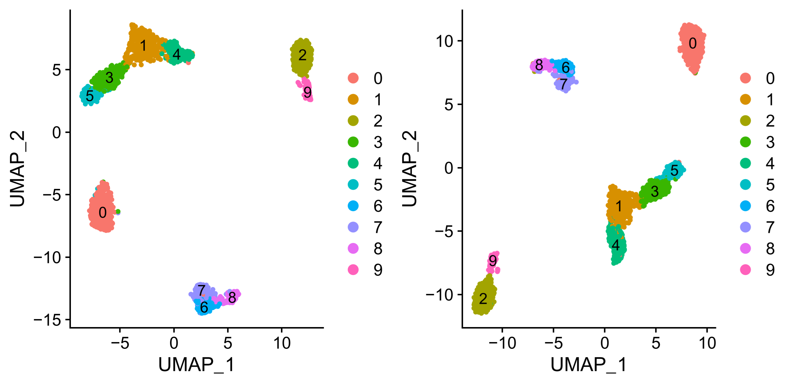
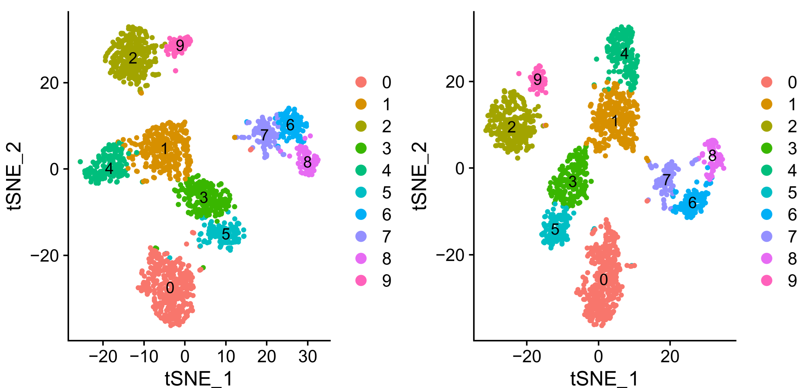
可以看到两种分析方法 umap 与 tsne 聚类效果不太相同，但是基本的聚类与分群是一致的

# 结语

就结果而言，两种分析方法的结果不完全相同，但也基本一致，本次笔记中用到的数据和代码已上传 github，在 ScRNAseq_code/compare 文件夹下，大家需要的可以下载试试

bioinformatics ScRNAseq